HTML5 Canvas 3D particles uniform distribution

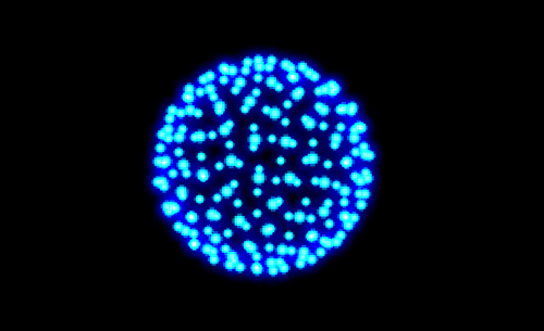
Yesterday Paul Rouget from Mozilla asked how to uniformly arrange points within a circle. There are a few existing algorithms to do this, but I was interested in seeing if I could use simple physics to create a stable system to distribute the particles evenly.

In the end I don’t think Paul could use them, (although I put him in touch with Mario who came up with slick solutions) but I enjoyed the process and found the results very pleasing!

Click on each thumbnail to see the effects in action. Tip : click to make more particles!

So how did I go about making this system?

I searched the dark recesses of my mind for a recollection of Robert Hodgin explaining the physics for his Magnetosphere : I needed to build a similar system where all particles repel each other.

To start with, I made a simple particle system with position, velocity and drag, explained in these two tutorials here and here if you need a refresher.

I’m using my own Vector object to store position and velocity. Vectors are critical to this type of visual programming, and if you haven’t used them before, it’s worth spending some time getting your head around them. Try this tutorial (based around Processing but still relevant).

Once we have that running we check all the particles against each other. We have an array of particle objects and we iterate through them in a nested loop :

for (i=0; i<particles.length-1; i++){

	var p1 = particles[i]; // the first particle

	for(j=i+1; j<particles.length; j++) {

		var p2 = particles[j]; // the second particle
		// compare p1 to p2 here... 

	}
}

If we have 5 particles :

0 1 2 3 4

The first time around the inner loop i will be 0 and j will go from 1 to 4 :

i  : 0 0 0 0  
j  : 1 2 3 4

the second time around :

i  : 1 1 1 
j  : 2 3 4 

third time :

i  : 2 2
j  : 3 4

final time :

i  : 3
j  : 4

For each comparison we work out the repulsion between the two particles: the closer they are, the more they repel, and we’ll store this value in repelforce vector. First, we set this to the vector between p1 and p2 :

 
repelforce.copyFrom(p2.position); 
repelforce.minusEq(p1.position); 

then we get the length or magnitude of that vector :

 
mag = repelforce.magnitude();

We calculate the repel force strength by subtracting the magnitude from 50 : the resulting value increases the closer the particles are.

 
repelstrength = 50-mag; 

If the force is less than 0, it means that the particles are further than 50 pixels apart, and no force should be applied. Otherwise, we have to work out a repelforce vector to apply to each particle’s velocity.

To do this, we divide the repelforce vector by its magnitude. This process is known as normalisation and it returns a unit vector : a vector with the same angle as before but with a length of 1.

 
repelforce.divideEq(mag); 

The great thing about unit vectors is that you can multiply them by any value to get a vector with a length of that value. So if we multiply it by our repelstrength, we’ll have our repelforce vector :

repelforce.multiplyEq(repelstrength); 

Except, we need to multiply that force by a small amount to make it less intense.

repelforce.multiplyEq(repelstrength*0.025); 

If we want our particles to repel more use a number higher than 0.025, if you want it to be more subtle go lower. I played around with this value until it seemed to work well.

Of course this division and multiplication can be combined into one call so

 
repelforce.divideEq(mag); 
repelforce.multiplyEq(repelstrength*0.025); 

can be simplified into :

 
repelforce.multiplyEq(repelstrength*0.025/mag); 

Each particle object has a force vector that we use to add up all the various forces for every frame update. As the force currently works in the direction from p1 to p2 it can be added to p2’s force to push it away from p1 :

 
p2.force.plusEq(repelforce);

We want p1 to go the opposite direction, so we subtract it from p1’s force:

 
p1.force.minusEq(repelforce); 

All that’s left is a very similar calculation of a force that stops the particles getting too far from the centre and we have a system! :

See it in action here.

The great thing about vector maths is that it also works in 3D with no changes at all! So a quick conversion into three.js and we have this :

See it in action here.

It seemed a bit chaotic so forced the particles onto the surface of a sphere:

See it in action here.
(Particle image courtesy of Mr.doob’s additive blend three.js particle example)

Wow. It’s taken me all afternoon to explain this, and I’m not entirely sure I’ve done that good a job! Please feel free to ask questions, and if you know this stuff well, perhaps you could point out where I could have explained things better.